01: Simulator Demo — Mutation-Selection Model

Background: Extending Fisher's Fundamental Theorem

This notebook implements an individual-based simulator for the mutation-selection model described in Basener & Sanford (2018). That paper extends Fisher's Fundamental Theorem of Natural Selection (FTNS) to rigorously account for the effects of mutations. Fisher's original theorem states that the rate of change in mean fitness equals the genetic variance in fitness: d(m̄)/dt = Var(m). Because variance is non-negative, this implies selection always increases mean fitness. Fisher assumed mutations would simply replenish genetic variance, leading to perpetual fitness increase.

Basener & Sanford proved a more complete result (their Theorem 2) that adds a mutational effects term:

d(m̄)/dt ≈ Var(m) + μ · E_g[s] · b̄

where:

Var(m) ≥ 0: genetic variance in fitness — Fisher's original term, always pushes fitness upward.
μ: per-birth mutation rate.
E_g[s]: mean fitness effect of a new mutation. Empirically negative, since the vast majority of mutations are deleterious.
b̄: mean per-capita birth rate.

Because E_g[s] is typically negative, the mutational term creates a drag on fitness that opposes selection. The critical condition for fitness increase is: Var(m) > μ |E_g[s]| b̄. When reversed, mutational meltdown occurs — fitness declines despite natural selection still operating. This contradicts Fisher's corollary that mutations plus selection necessarily increase fitness.

The theorem gives instantaneous rates of change, but the actual dynamics in finite populations with stochastic effects (genetic drift, Muller's ratchet, demographic noise) require simulation. That is the purpose of this notebook.

Simulator Parameters and Their Biological Meaning

Each parameter in the simulator corresponds to a biological quantity in the Basener-Sanford model. The table below shows how the computational parameters map to the terms in the theorem.

1. Default Parameter Trajectories

Parameter	Symbol in theorem	Default	Biological meaning
`b0`	b̄	2.0	Baseline offspring per parent (mean per-capita birth rate). Appears directly in the mutational drag term μ · E_g[s] · b̄. Higher birth rates amplify the effect of mutations because more births mean more mutational events per generation.
`mu`	μ	0.1	Per-offspring mutation probability. This is the mutation rate in the theorem. Each offspring independently acquires a mutation with this probability.
`gamma_shape`	—	2.0	Shape of the gamma-distributed DFE (Distribution of Fitness Effects). Values < 1 produce an L-shaped distribution with many very slightly deleterious mutations (VSDMs) and few large-effect mutations, matching empirical data (Kimura 1979, Keightley & Lynch 2003). Values ≥ 1 give a more bell-shaped distribution.
`gamma_scale`	—	0.004	Scale of the gamma DFE. Together with shape, determines the mean deleterious effect: E_g[s] ≈ −shape × scale (for the deleterious fraction). Larger scale means each mutation has a bigger fitness cost on average.
`p_beneficial`	—	0.003	Fraction of mutations that increase fitness. Empirically very small (~0.1–1%). The overwhelming majority of mutations are neutral-to-deleterious.
`sigma_env_ind`	—	0.01	Environmental noise on fitness expression. Represents the fact that the same genotype may express different phenotypic fitness depending on environmental conditions.
`K`	—	1000	Carrying capacity. Density-dependent regulation prevents unlimited growth and determines effective population size relevant to genetic drift.
`init_fitness`	m_i	0.044	Initial Malthusian fitness parameter (m_i = b_i − d_i, the difference between individual birth and death rates).

Default parameter simulation trajectories

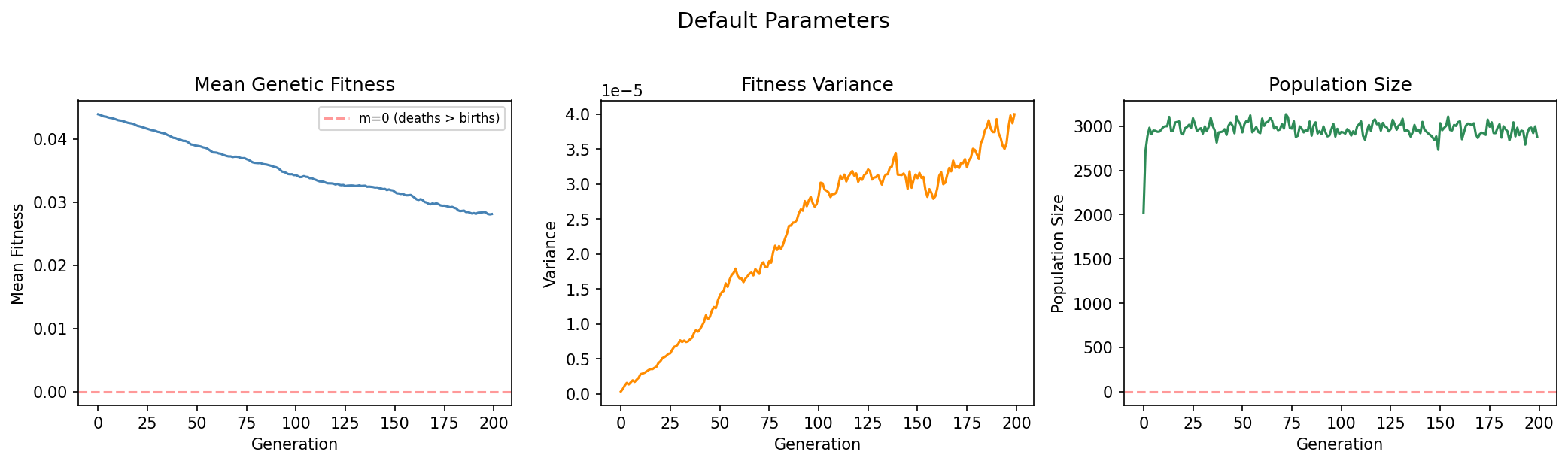
Figure 1: Single simulation with default parameters. Three panels track the population over 200 generations. Left — Mean fitness (m̄): This is the central quantity in the Basener-Sanford theorem. Its trajectory reveals whether the genetic variance term Var(m) or the mutational drag term μ |E_g[s]| b̄ dominates. With default parameters (mu=0.1, gamma_shape=2.0, gamma_scale=0.004), the population shows moderate fitness decline as deleterious mutations accumulate faster than selection can purge them — the mutational drag exceeds the variance-driven selection response. Center — Fitness variance (Var(m)): This is Fisher's term, the fuel for natural selection. Without genetic variance, selection has no material to act on. Note how variance initially increases as mutations spread fitness values apart, but may eventually decline if the population contracts or becomes uniformly degraded. Right — Population size: Reflects the demographic consequences of fitness changes. As mean Malthusian fitness (m = b − d) declines, per-capita growth rate decreases, eventually causing population contraction. This contraction further weakens selection (smaller populations experience stronger drift), potentially initiating a feedback loop toward meltdown.

2. Three Dynamical Regimes

The critical condition from Basener & Sanford's theorem determines which dynamical regime a population enters:

We demonstrate this by running three scenarios that differ in mutation rate (μ) and DFE parameters (gamma_shape, gamma_scale), placing each population at a different position relative to the critical threshold.

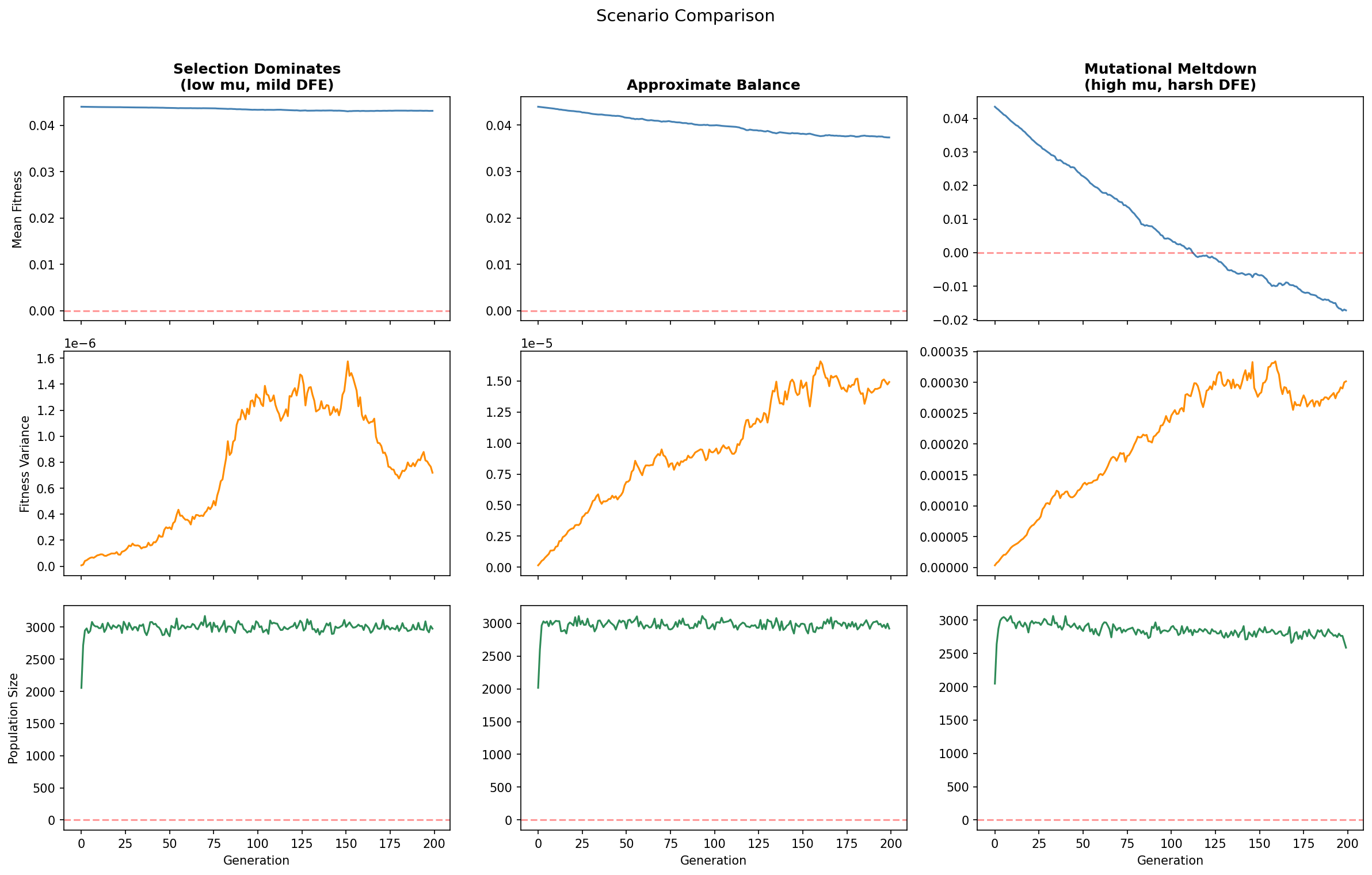
Figure 2: The three dynamical regimes predicted by the extended theorem.

Selection Dominates (mu=0.01, mild DFE): This is the regime Fisher implicitly assumed was universal. The mutational drag μ |E_g[s]| b̄ is small relative to Var(m), so selection efficiently purges deleterious mutations. Mean fitness is sustained or increases. The population remains near carrying capacity.
Approximate Balance (mu=0.05, moderate DFE): At the critical threshold, Fisher's variance term and the mutational drag roughly cancel. Mean fitness fluctuates stochastically around its initial value. This is a phase transition — small changes in parameters can tip the population toward adaptation or decline.
Mutational Meltdown (mu=0.2, harsh DFE): The mutational drag overwhelms selection. Mean fitness declines relentlessly. This regime is what empirical DFE data — strongly L-shaped, dominated by very slightly deleterious mutations (VSDMs; Kimura 1979, Keightley & Lynch 2003) — suggests may be more biologically common than Fisher assumed. VSDMs are particularly dangerous: each individual mutation is too small for selection to act on efficiently, yet they accumulate relentlessly (Kondrashov 1995). Declining fitness reduces population size, which weakens selection further (more drift in smaller populations), creating a positive feedback loop — mutational meltdown in the sense of Lynch & Gabriel (1990), closely related to Muller's ratchet.

The biological significance: the outcome is not a foregone conclusion. Whether a population adapts or decays depends quantitatively on the mutation rate, the shape of the DFE, and the population size — all empirical questions, not theoretical certainties. This is the central insight of the Basener-Sanford paper.

3. Stochastic Replication — Why Bayesian Inference Is Needed

The simulator models finite populations, unlike the infinite-population deterministic models in Section 2.2 of the paper. In finite populations, several stochastic effects are important:

The consequence: identical parameters produce different trajectories. A single simulation is one draw from a stochastic process. To characterize the distribution of outcomes, we run many replicates in parallel.

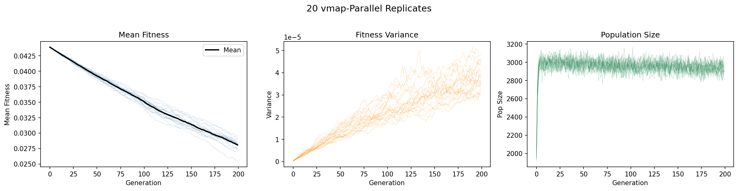
Figure 3: Twenty independent replicates run in parallel via jax.vmap. All twenty replicates use identical parameters but different random seeds. Thin colored lines show individual replicates; the black line shows the ensemble mean. Left — Mean fitness: Note the substantial spread across replicates. Some populations experience more severe fitness decline than others, purely due to stochastic effects. The variance across replicates is not experimental error — it is intrinsic to the biological process. Center — Fitness variance: The fuel for selection also varies across replicates. Populations that by chance accumulate more mutations may have higher variance (more material for selection) but also lower mean fitness. Right — Population size: Demographic consequences of the stochastic fitness trajectories. Some replicates may approach carrying capacity while others decline.

This stochastic variability is precisely why Bayesian inference is needed in notebooks 02–06. If the simulator were deterministic, we could find parameters that exactly reproduce an observed dataset. But because the same parameters produce a range of outcomes, we must ask: "What distribution of parameters is consistent with the observed data, given the intrinsic noise of the process?" This is the question that Approximate Bayesian Computation (notebook 02), Bayesian Synthetic Likelihood (notebook 03), and Simulation-Based Inference (notebooks 04b, 04c) are designed to answer.

What We Learn

Summary: Simulation Confirms Theory

The simulator computationally confirms the three dynamical regimes predicted by Basener & Sanford's extended theorem. The three regimes map directly to the critical condition Var(m) vs. μ |E_g[s]| b̄:

Selection dominates when Var(m) exceeds the mutational drag — Fisher's implicit assumption, but not guaranteed by biology.
Approximate balance at the phase transition — the population's fate is sensitive to stochastic fluctuations.
Mutational meltdown when mutational drag exceeds Var(m) — what empirical DFE data suggests may be the more common regime.

The simulator adds two critical capabilities beyond the analytical theorem: finite population effects (drift, Muller's ratchet, demographic stochasticity) and long-term trajectory dynamics (not just instantaneous rates of change). The stochastic variability across replicates motivates the Bayesian inference methods developed in notebooks 02–06, which tackle the inverse problem: given observed population trajectories, what can we infer about the underlying mutation rate, DFE shape, and other biological parameters?

01: Simulator Demo — The Basener-Sanford Mutation-Selection Model